KV Cache from First Principles
A clear first-principles guide to KV cache: why it exists, how it works, and what tradeoffs matter in real production systems.

On this page
KV Cache from First Principles
A simple idea powers fast follow-up answers in modern LLMs: do not recompute what is already stable. This guide keeps the language simple, removes extra noise, and focuses on the decisions that matter when you build real systems.
See how the model reads old context during generation.
See how each new token gets added to cache.
See what limits performance first in real systems.
1. How Transformers Create The Bottleneck
Every LLM token is represented as numbers, then projected into three vectors: Query (Q), Key (K), and Value (V). During attention, each new token compares its query with keys from prior tokens and combines the corresponding values. That gives context-aware output, but it is expensive because generation is autoregressive: one token at a time. You cannot skip steps because token t+1 depends on token t. In long prompts, this means the model repeatedly touches earlier context. That repeated touching is not automatically waste, but recomputing unchanged K/V states is. This is where the performance bottleneck starts.
What this token wants to find in older tokens.
A label used to decide if a token is relevant.
The actual information used for the output.
Query_i = Token_i x W_Q
Key_i   = Token_i x W_K
Value_i = Token_i x W_V
Attention(i -> j) = dot(Query_i, Key_j) / sqrt(d)
Output_i = sum_j softmax(Attention(i -> j)) * Value_j
Each new token asks a question using Q, checks old tokens using K, and pulls useful info using V. The math is simple. The key systems idea is simpler: if old K and V do not change, do not recompute them.
2. Why Naive Decoding Wastes Massive Compute
Assume the prompt is The capital of France is. At the first decode step, the model computes K/V for those prompt tokens and predicts Paris. At the second step, it predicts a period. In a naive pipeline, it recomputes K/V for the same old prompt tokens again, even though those tokens and positions are unchanged. At the third step, same pattern. This redundancy grows with sequence length, so wasted work becomes a major latency and cost driver. The core issue is not attention itself, but repeated re-derivation of stable states. If a system keeps doing identical work at every step, it will always be slower than necessary.
Redundant compute grows with context length.
Same model behavior, much less repeated work.
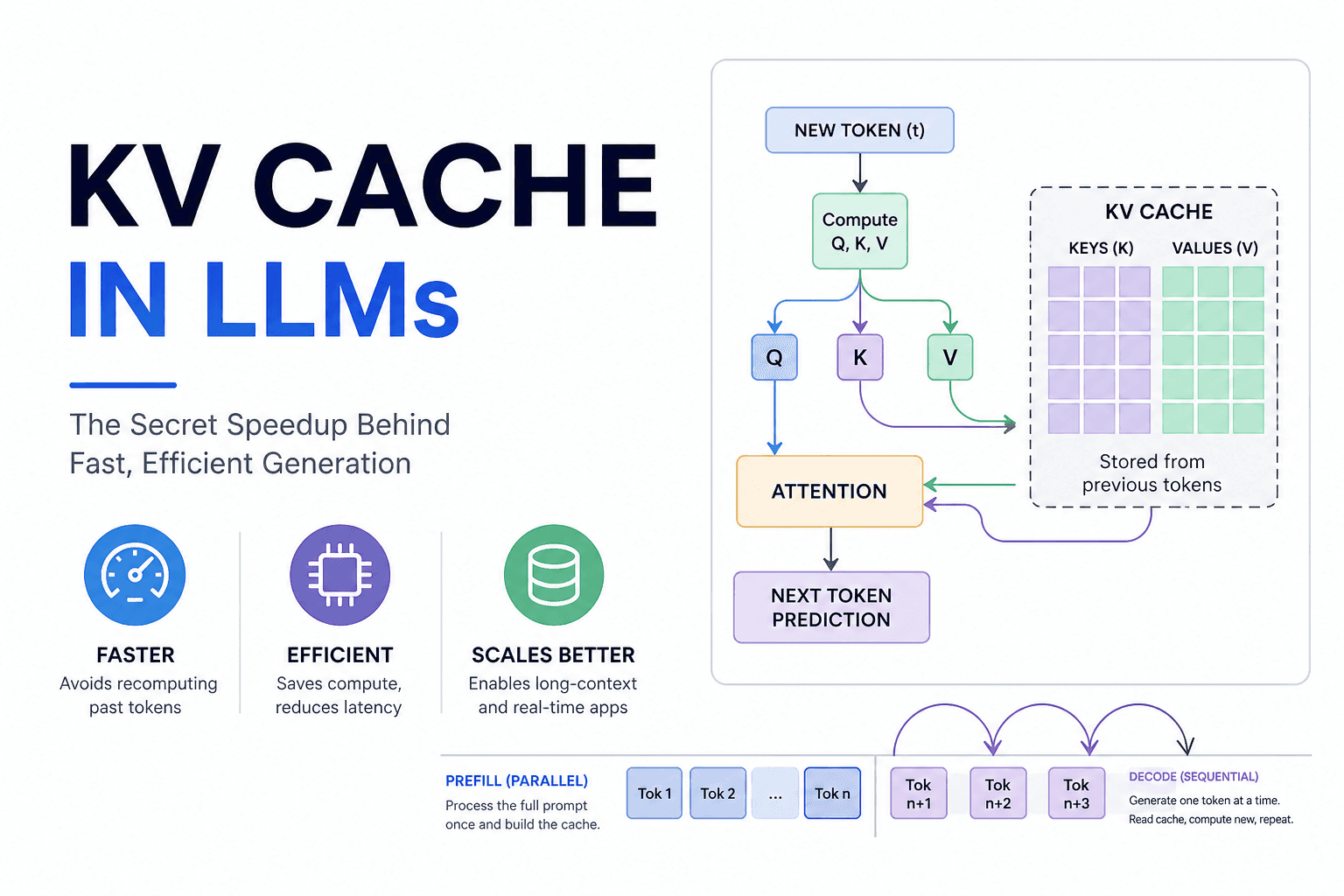
Visual Checkpoint: Prefill vs Decode Timeline
The model reads the full prompt at once and builds K/V for all prompt tokens. This step is fast on GPUs because many operations run in parallel.
The model then generates one token at a time. Each step reads cache and adds one new state. For long context, memory movement becomes the main limit.
3. KV Cache Mechanism, In One Practical Mental Model
KV cache stores per-layer keys and values for tokens that are already processed. The next token still computes a fresh query, but instead of recomputing every previous key/value, it reads prior K/V from cache and appends only the new token state. This is exact for causal decoding because past token states do not change after they are computed in that sequence context. You can think of it as memoization for attention internals. The model is still doing attention over full history; it is simply not wasting compute rebuilding stable intermediate outputs. This is the single biggest reason multi-turn generation feels responsive in deployed systems.
Load old K/V for previous tokens.
Compute K/V only for the new token.
Append cache, run attention, predict next token.
# Simplified decode step
for L in layers:
  k_new = x_new @ W_K[L]
  v_new = x_new @ W_V[L]

  k_all = concat(cache[L].keys, k_new)
  v_all = concat(cache[L].values, v_new)

  y_new = attention(q_new, k_all, v_all)

  cache[L].keys.append(k_new)
  cache[L].values.append(v_new)
4. Tradeoffs: Compute Savings vs Memory Pressure
KV cache does not come free. It shifts pressure from repeated math to memory capacity and memory bandwidth. As context length increases, cache size grows linearly with tokens, layers, and head dimensions. During decode, each step needs to read large cached tensors, so long-context serving often becomes memory-bandwidth bound instead of compute-bound. This is why GPU VRAM limits, cache layout, and allocation strategy matter so much in production. In practice, teams optimize both sides: reduce redundant compute with caching while controlling memory via attention variants, cache quantization, and better paging strategies. High-quality inference engineering is mostly this balancing act.
| Concern | Impact | Typical Mitigation |
|---|---|---|
| Cache size growth | Fewer concurrent requests per GPU | GQA/MQA, quantized KV |
| Memory bandwidth at decode | Token generation slows at long context | Better kernel and cache layout |
| Fragmentation | Wasted VRAM and unstable throughput | PagedAttention-style blocks |
| Prefix mismatch | Cache reuse drops in chat turns | Stable prompt templates |
5. Production Extensions That Actually Matter
Real serving systems go beyond baseline KV cache. Grouped-Query Attention reduces memory by sharing K/V across groups of heads, and Multi-Query Attention pushes this further by sharing across all heads. PagedAttention improves memory efficiency by managing cache in fixed blocks instead of giant contiguous regions, which reduces fragmentation and improves throughput under mixed workloads. Prefix caching reuses long shared system prefixes across many calls, avoiding repeated prefill cost. KV quantization stores cache with lower precision to reduce VRAM usage while preserving quality in many tasks. These methods are practical, widely used, and often decisive for cost and latency targets.
Visual Checkpoint: Optimization Map
6. Why This Changes Real Products
KV cache is not just a low-level trick. It changes product feasibility. Without it, long-context assistants, code copilots, and document chat systems would be slower and costlier, especially in follow-up turns where users expect near-instant replies. Better cache systems reduce inference cost per useful token, which translates into lower API bills or higher quality at the same budget. They also enable more stable user experience under load because the system wastes less repeated work. The big picture is simple: smart memory reuse turns transformer inference from a lab demo into something production teams can scale with predictable latency.
7. Open Problems And A Practical Checklist
The field is still moving fast. Long-context models still struggle with mid-context retrieval quality, cache eviction strategies are still heuristic-heavy, and speculative decoding adds complexity when accepted and rejected draft tokens must keep cache state consistent. Cross-request semantic caching is promising but hard because token-order dependence is strict. For practitioners, the best approach is disciplined measurement: separate prefill and decode metrics, track cache hit behavior for shared prefixes, watch bandwidth saturation, and verify quality after quantization. Keep the architecture simple first, then add optimizations in layers so regressions remain debuggable.
- Measure prefill latency and decode tokens/sec separately.
- Keep prompt templates stable to maximize prefix reuse.
- Profile VRAM and memory bandwidth, not just FLOPs.
- Introduce GQA/MQA and quantization only with quality checks.
- Validate behavior under real multi-turn traffic, not synthetic single-turn tests.
KV cache is a simple idea with serious consequences: compute once, reuse many times. The models did not become practical by magic. They became practical because systems engineering removed repeated work without changing model intelligence.