HNSW: How a Vector Database Really Searches

Modern AI search works by turning meaning into position. Every document becomes a point in space, arranged so that things meaning similar things sit near each other. To find documents about refunds, you turn "refunds" into a point and look for its neighbours.

The catch is that the space has hundreds of dimensions, not two, and there may be ten million points in it.

The obvious approach — measure the distance to all ten million and sort — is correct, easy, and far too slow. Every serious system does something else, and that something else is almost certainly HNSW. Understanding it changes how you tune a search system, because every setting it exposes is a position on a curve you should be choosing deliberately.

1. Why the normal tricks fail

For a sorted list, finding things is easy. For a map — two dimensions — it is still easy: chop the map into quarters, then quarters of quarters, and to find something near a point you only look in nearby squares and ignore the rest. That is how computer graphics works, and the structures are beautiful.

They stop working around ten dimensions. Embeddings have hundreds.

The reason has a name — the curse of dimensionality — and a specific mechanism worth stating, because it is not obvious.

Chopping space into regions only helps if you can prove an entire region is too far away to bother with, and skip it. That proof needs the region to be clearly further than your current best candidate.

In high dimensions it never is. As dimensions increase, the distances from any point to all the others bunch up into a narrow band. The nearest neighbour is only slightly nearer than a typical one. So the skipping condition almost never holds, and your elegant structure quietly degrades into checking everything, with extra bookkeeping.

That is not a flaw in the structure. It is a property of high-dimensional space, and it defeats every method built on carving space into regions.

2. Stop carving. Start connecting.

The idea that works comes from social networks.

You have probably heard that any two people are connected by about six handshakes. The remarkable part is not that a short path exists. It is that you can find it without a map. Nobody knows the global social graph. You just forward the message to whoever you know who seems closest to the target, and it gets there.

That works because your friends are a mix: mostly people nearby, plus a few far away. The nearby ones let you home in; the far ones let you cross huge distances in one step.

Apply that to search. Build a network where each stored point is connected to a handful of its near neighbours. To search, start anywhere and repeatedly step to whichever neighbour is closer to what you are looking for. Stop when no neighbour is an improvement.

The long-distance links are what make this fast. Without them, you shuffle along local structure and it takes forever to cross the dataset.

But a flat network like this has a problem: most of your steps get spent in the early, coarse phase, and the step sizes are not well controlled.

3. The layers, borrowed from express trains

Yu. A. Malkov and D. A. Yashunin's contribution, in Efficient and robust approximate nearest neighbor search using Hierarchical Navigable Small World graphs (2016), was to organise those step sizes by separating them into layers.

Think of a metro system. The bottom layer is the local line stopping at every station. Above it, an express line stopping at every fifth station. Above that, an intercity line with four stops in the whole country.

To travel, you start on the fastest line, ride until you overshoot, drop down a level, repeat. Coarse to fine.

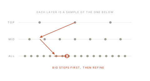
HNSW builds exactly this. The bottom layer contains every point. Each layer above holds a random sample of the one below, getting sparser fast — so the top layer has a handful of points and the bottom has all ten million.

Searching runs top-down:

1. Enter at the single point in the top layer.
2. Step greedily through that layer until no neighbour is closer.
3. Drop to the next layer, starting from where you stopped.
4. Repeat down to the bottom, where you search a bit wider and collect your results.

The upper layers are sparse, so their links span huge distances and each step covers a lot of ground. The lower layers are dense and refine. Step size falls by roughly a constant factor per layer — which is exactly what produces the paper's logarithmic scaling: ten times more data costs you only a couple more steps.

4. Building it is the same algorithm

Adding a point:

1. Roll dice to pick its top layer — most points get only the bottom, a few get high.
2. Search from the very top down to that layer to find where it belongs.
3. In each layer from its top down to the bottom, find the best candidates nearby and connect to the closest $M$ of them.
4. Links go both ways, so the neighbours gain a connection too. If any now has too many, drop its worst.

Step 4 is where the quality lives, and the rule is subtler than "drop the furthest."

HNSW prefers a spread-out set of neighbours over a merely close one: a candidate is kept if it is closer to this point than to any neighbour already chosen. The effect is to keep links pointing in different directions rather than bunching them all on one side.

That spread is what keeps the network navigable. A point whose every link goes the same way is a dead end for anyone arriving from elsewhere — and in real data, which comes in clumps, naive nearest-neighbour links produce exactly that.

5. The three settings you actually tune

Every vector database exposes these, usually under these names.

$M$ — links per point. Higher gives better recall and uses more memory, because the network itself has to be held in memory. Typical values are 16 to 64. For large collections the links can rival the data in size.

$\mathrm{efConstruction}$ — how hard to look while building. Higher gives a better network and slower building. It costs nothing at search time — this is effort spent once that pays off on every future search, so it is usually worth setting generously.

$\mathrm{ef}$ — how hard to look while searching. The live dial. Higher gives better recall and slower searches, and you can change it per query without rebuilding anything. This is the one to expose to your application: an as-you-type suggestion box and an overnight batch job want very different values.

6. Filtering is harder than it looks

The single most common real requirement — find similar documents, but only this customer's, in English, from this year — is genuinely awkward here, and it is worth knowing why before you design around it.

Filter afterwards. Search normally, then throw away non-matching results. Simple, and it collapses when the filter is picky: you ask for 10, fetch 100, and 3 match. You cannot know in advance how much to over-fetch.

Filter first. Work out the matching subset, then search within it. Correct, but the network's links connect everything. Restricted to a subset, your walk keeps trying to step through excluded points — and if the subset is small, the network is effectively broken into islands. At that point simply checking every point in the subset is genuinely faster, and good implementations switch to exactly that.

Filter while walking. What mature systems do: consult the filter during the walk and only step to permitted points, with extra tricks to keep things connected. Qdrant, for example, builds additional links based on the labels so that heavily-filtered searches stay navigable.

The practical consequence: if every search is always scoped to one customer, separate collections per customer often beat one collection with a filter. The filter costs you on every query; the separation is free.

7. What this changes about using one

Four things follow directly.

The index is a network held in memory, not a file you read from disk. Capacity planning must count the data plus the links, and the links are not a rounding error.

Recall is a dial, not a fact. If search quality is poor, check ef first — you may be running a default tuned for speed.

"Everything within this distance" is not supported. HNSW answers "the nearest handful." Systems offering a radius search do it by over-fetching and filtering, with no guarantee of completeness.

Build time is not wasted time. A generous build setting produces a network that is better on every single search for the life of the index.

The idea underneath is worth carrying beyond search: when dividing a space stops working, stop dividing it and start connecting it. Navigation succeeds where subdivision fails, because a good network does not need to understand the geometry. It only needs enough well-chosen links that always-step-closer adds up to arriving.

Sources

• Malkov, Yashunin — Efficient and robust approximate nearest neighbor search using Hierarchical Navigable Small World graphs, 2016
• Malkov, Ponomarenko, Logvinov, Krylov — Approximate nearest neighbor algorithm based on navigable small world graphs, Information Systems, 2014
• Pugh — Skip Lists: A Probabilistic Alternative to Balanced Trees, CACM, 1990